
reference: PyTorch Loss Functions: The Ultimate Guide – neptune.ai
Your neural networks can do a lot of different tasks. Whether it’s classifying data, like grouping pictures of animals into cats and dogs, regression tasks, like predicting monthly revenues, or anything else. Every task has a different output and needs a different type of loss function.
The way you configure your loss functions can make or break the performance of your algorithm. By correctly configuring the loss function, you can make sure your model will work how you want it to.
Luckily for us, there are loss functions we can use to make the most of machine learning tasks.
In this article, we’ll talk about popular loss functions in PyTorch, and about building custom loss functions. Once you’re done reading, you should know which one to choose for your project.
May be useful
Check how you can monitor your PyTorch model training and keep track of all model-building metadata with Neptune + PyTorch integration.
What are the loss functions?
Before we jump into PyTorch specifics, let’s refresh our memory of what loss functions are.
Loss functions are used to gauge the error between the prediction output and the provided target value. A loss function tells us how far the algorithm model is from realizing the expected outcome. The word ‘loss’ means the penalty that the model gets for failing to yield the desired results.
For example, a loss function (let’s call it J) can take the following two parameters:
- Predicted output (y_pred)
- Target value (y)

This function will determine your model’s performance by comparing its predicted output with the expected output. If the deviation between y_pred and y is very large, the loss value will be very high.
If the deviation is small or the values are nearly identical, it’ll output a very low loss value. Therefore, you need to use a loss function that can penalize a model properly when it is training on the provided dataset.
Loss functions change based on the problem statement that your algorithm is trying to solve.
How to add PyTorch loss functions?
PyTorch’s torch.nn module has multiple standard loss functions that you can use in your project.
To add them, you need to first import the libraries:
import torch
import torch.nn as nn
Next, define the type of loss you want to use. Here’s how to define the mean absolute error loss function:
loss = nn.L1Loss()After adding a function, you can use it to accomplish your specific task.
Which loss functions are available in PyTorch?
Broadly speaking, loss functions in PyTorch are divided into two main categories: regression losses and classification losses.
Regression loss functions are used when the model is predicting a continuous value, like the age of a person.
Classification loss functions are used when the model is predicting a discrete value, such as whether an email is spam or not.
Ranking loss functions are used when the model is predicting the relative distances between inputs, such as ranking products according to their relevance on an e-commerce search page.
Now we’ll explore the different types of loss functions in PyTorch, and how to use them:
- Mean Absolute Error Loss
- Mean Squared Error Loss
- Negative Log-Likelihood Loss
- Cross-Entropy Loss
- Hinge Embedding Loss
- Margin Ranking Loss
- Triplet Margin Loss
- Kullback-Leibler divergence
1. PyTorch Mean Absolute Error (L1 Loss Function)
torch.nn.L1LossThe Mean Absolute Error (MAE), also called L1 Loss, computes the average of the sum of absolute differences between actual values and predicted values.
It checks the size of errors in a set of predicted values, without caring about their positive or negative direction. If the absolute values of the errors are not used, then negative values could cancel out the positive values.
The Pytorch L1 Loss is expressed as:
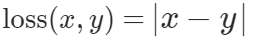
x represents the actual value and y the predicted value.
When could it be used?
- Regression problems, especially when the distribution of the target variable has outliers, such as small or big values that are a great distance from the mean value. It is considered to be more robust to outliers.
Example
import torch
import torch.nn as nn

input = torch.randn(3, 5, requires_grad=True)
target = torch.randn(3, 5)

mae_loss = nn.L1Loss()
output = mae_loss(input, target)
output.backward()

print('input: ', input)
print('target: ', target)
print('output: ', output)
###################### OUTPUT ######################
input: tensor([[ 0.2423, 2.0117, -0.0648, -0.0672, -0.1567],
[-0.2198, -1.4090, 1.3972, -0.7907, -1.0242],
[ 0.6674, -0.2657, -0.9298, 1.0873, 1.6587]], requires_grad=True)
target: tensor([[-0.7271, -0.6048, 1.7069, -1.5939, 0.1023],
[-0.7733, -0.7241, 0.3062, 0.9830, 0.4515],
[-0.4787, 1.3675, -0.7110, 2.0257, -0.9578]])
output: tensor(1.2850, grad_fn=<L1LossBackward>)2. PyTorch Mean Squared Error Loss Function
torch.nn.MSELossThe Mean Squared Error (MSE), also called L2 Loss, computes the average of the squared differences between actual values and predicted values.
Pytorch MSE Loss always outputs a positive result, regardless of the sign of actual and predicted values. To enhance the accuracy of the model, you should try to reduce the L2 Loss—a perfect value is 0.0.
The squaring implies that larger mistakes produce even larger errors than smaller ones. If the classifier is off by 100, the error is 10,000. If it’s off by 0.1, the error is 0.01. This punishes the model for making big mistakes and encourages small mistakes.
The Pytorch L2 Loss is expressed as:
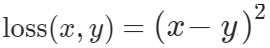
x represents the actual value and y the predicted value.
When could it be used?
- MSE is the default loss function for most Pytorch regression problems.
Example
import torch
import torch.nn as nn

input = torch.randn(3, 5, requires_grad=True)
target = torch.randn(3, 5)
mse_loss = nn.MSELoss()
output = mse_loss(input, target)
output.backward()

print('input: ', input)
print('target: ', target)
print('output: ', output)
###################### OUTPUT ######################


input:  tensor([[ 0.3177,  1.1312, -0.8966, -0.0772,  2.2488],
        [ 0.2391,  0.1840, -1.2232,  0.2017,  0.9083],
        [-0.0057, -3.0228,  0.0529,  0.4084, -0.0084]], requires_grad=True)
target:  tensor([[ 0.2767,  0.0823,  1.0074,  0.6112, -0.1848],
        [ 2.6384, -1.4199,  1.2608,  1.8084,  0.6511],
        [ 0.2333, -0.9921,  1.5340,  0.3703, -0.5324]])
output:  tensor(2.3280, grad_fn=<MseLossBackward>)
3. PyTorch Negative Log-Likelihood Loss Function
torch.nn.NLLLossThe Negative Log-Likelihood Loss function (NLL) is applied only on models with the softmax function as an output activation layer. Softmax refers to an activation function that calculates the normalized exponential function of every unit in the layer.
The Softmax function is expressed as:
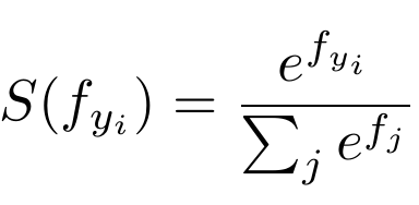
The function takes an input vector of size N, and then modifies the values such that every one of them falls between 0 and 1. Furthermore, it normalizes the output such that the sum of the N values of the vector equals to 1.
NLL uses a negative connotation since the probabilities (or likelihoods) vary between zero and one, and the logarithms of values in this range are negative. In the end, the loss value becomes positive.
In NLL, minimizing the loss function assists us get a better output. The negative log likelihood is retrieved from approximating the maximum likelihood estimation (MLE). This means that we try to maximize the model’s log likelihood, and as a result, minimize the NLL.
In NLL, the model is punished for making the correct prediction with smaller probabilities and encouraged for making the prediction with higher probabilities. The logarithm does the punishment.
NLL does not only care about the prediction being correct but also about the model being certain about the prediction with a high score.
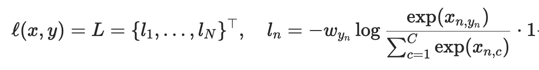
The Pytorch NLL Loss is expressed as:
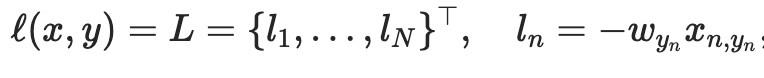
where x is the input, y is the target, w is the weight, and N is the batch size.
When could it be used?
- Multi-class classification problems
Example
import torch
import torch.nn as nn

# size of input (N x C) is = 3 x 5
input = torch.randn(3, 5, requires_grad=True)
# every element in target should have 0 <= value < C
target = torch.tensor([1, 0, 4])

m = nn.LogSoftmax(dim=1)
nll_loss = nn.NLLLoss()
output = nll_loss(m(input), target)
output.backward()

print('input: ', input)
print('target: ', target)
print('output: ', output)
###################### OUTPUT ######################
input: tensor([[ 1.6430, -1.1819, 0.8667, -0.5352, 0.2585],
[ 0.8617, -0.1880, -0.3865, 0.7368, -0.5482],
[-0.9189, -0.1265, 1.1291, 0.0155, -2.6702]], requires_grad=True)
target: tensor([1, 0, 4])
output: tensor(2.9472, grad_fn=<NllLossBackward>)4. PyTorch Cross-Entropy Loss Function
torch.nn.CrossEntropyLoss
This loss function computes the difference between two probability distributions for a provided set of occurrences or random variables.
It is used to work out a score that summarizes the average difference between the predicted values and the actual values. To enhance the accuracy of the model, you should try to minimize the score—the cross-entropy score is between 0 and 1, and a perfect value is 0.
Other loss functions, like the squared loss, punish incorrect predictions. Cross-Entropy penalizes greatly for being very confident and wrong.
Unlike the Negative Log-Likelihood Loss, which doesn’t punish based on prediction confidence, Cross-Entropy punishes incorrect but confident predictions, as well as correct but less confident predictions.
The Cross-Entropy function has a wide range of variants, of which the most common type is the Binary Cross-Entropy (BCE). The BCE Loss is mainly used for binary classification models; that is, models having only 2 classes.
The Pytorch Cross-Entropy Loss is expressed as:
Where x is the input, y is the target, w is the weight, C is the number of classes, and N spans the mini-batch dimension.
When could it be used?
- Binary classification tasks, for which it’s the default loss function in Pytorch.
- Creating confident models—the prediction will be accurate and with a higher probability.
Example
import torch
import torch.nn as nn

input = torch.randn(3, 5, requires_grad=True)
target = torch.empty(3, dtype=torch.long).random_(5)

cross_entropy_loss = nn.CrossEntropyLoss()
output = cross_entropy_loss(input, target)
output.backward()

print('input: ', input)
print('target: ', target)
print('output: ', output)
###################### OUTPUT ######################
input: tensor([[ 0.1639, -1.2095, 0.0496, 1.1746, 0.9474],
[ 1.0429, 1.3255, -1.2967, 0.2183, 0.3562],
[-0.1680, 0.2891, 1.9272, 2.2542, 0.1844]], requires_grad=True)
target: tensor([4, 0, 3])
output: tensor(1.0393, grad_fn=<NllLossBackward>)5. PyTorch Hinge Embedding Loss Function
torch.nn.HingeEmbeddingLoss
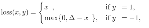
The Hinge Embedding Loss is used for computing the loss when there is an input tensor, x, and a labels tensor, y. Target values are between {1, -1}, which makes it good for binary classification tasks.
With the Hinge Loss function, you can give more error whenever a difference exists in the sign between the actual class values and the predicted class values. This motivates examples to have the right sign.
The Hinge Embedding Loss is expressed as:
When could it be used?
- Classification problems, especially when determining if two inputs are dissimilar or similar.
- Learning nonlinear embeddings or semi-supervised learning tasks.
Example
import torch
import torch.nn as nn

input = torch.randn(3, 5, requires_grad=True)
target = torch.randn(3, 5)

hinge_loss = nn.HingeEmbeddingLoss()
output = hinge_loss(input, target)
output.backward()

print('input: ', input)
print('target: ', target)
print('output: ', output)
###################### OUTPUT ######################
input: tensor([[ 0.1054, -0.4323, -0.0156, 0.8425, 0.1335],
[ 1.0882, -0.9221, 1.9434, 1.8930, -1.9206],
[ 1.5480, -1.9243, -0.8666, 0.1467, 1.8022]], requires_grad=True)
target: tensor([[-1.0748, 0.1622, -0.4852, -0.7273, 0.4342],
[-1.0646, -0.7334, 1.9260, -0.6870, -1.5155],
[-0.3828, -0.4476, -0.3003, 0.6489, -2.7488]])
output: tensor(1.2183, grad_fn=<MeanBackward0>)6. PyTorch Margin Ranking Loss Function
torch.nn.MarginRankingLoss
The Margin Ranking Loss computes a criterion to predict the relative distances between inputs. This is different from other loss functions, like MSE or Cross-Entropy, which learn to predict directly from a given set of inputs.
With the Margin Ranking Loss, you can calculate the loss provided there are inputs x1, x2, as well as a label tensor, y (containing 1 or -1).
When y == 1, the first input will be assumed as a larger value. It’ll be ranked higher than the second input. If y == -1, the second input will be ranked higher.
The Pytorch Margin Ranking Loss is expressed as:

When could it be used?
- Ranking problems
Example
import torch
import torch.nn as nn

input_one = torch.randn(3, requires_grad=True)
input_two = torch.randn(3, requires_grad=True)
target = torch.randn(3).sign()

ranking_loss = nn.MarginRankingLoss()
output = ranking_loss(input_one, input_two, target)
output.backward()

print('input one: ', input_one)
print('input two: ', input_two)
print('target: ', target)
print('output: ', output)
###################### OUTPUT ######################
input one: tensor([1.7669, 0.5297, 1.6898], requires_grad=True)
input two: tensor([ 0.1008, -0.2517, 0.1402], requires_grad=True)
target: tensor([-1., -1., -1.])
output: tensor(1.3324, grad_fn=<MeanBackward0>)7. PyTorch Triplet Margin Loss Function
torch.nn.TripletMarginLoss
The Triplet Margin Loss computes a criterion for measuring the triplet loss in models. With this loss function, you can calculate the loss provided there are input tensors, x1, x2, x3, as well as margin with a value greater than zero.
A triplet consists of a (anchor), p (positive examples), and n (negative examples).
The Pytorch Triplet Margin Loss is expressed as:

When could it be used?
- Determining the relative similarity existing between samples.
- It is used in content-based retrieval problems
Example
import torch
import torch.nn as nn
anchor = torch.randn(100, 128, requires_grad=True)
positive = torch.randn(100, 128, requires_grad=True)
negative = torch.randn(100, 128, requires_grad=True)

triplet_margin_loss = nn.TripletMarginLoss(margin=1.0, p=2)
output = triplet_margin_loss(anchor, positive, negative)
output.backward()

print('anchor: ', anchor)
print('positive: ', positive)
print('negative: ', negative)
print('output: ', output)
###################### OUTPUT ######################

anchor:  tensor([[ 0.6152, -0.2224,  2.2029,  <strong>...</strong>, -0.6894,  0.1641,  1.7254],
        [ 1.3034, -1.0999,  0.1705,  <strong>...</strong>,  0.4506, -0.2095, -0.8019],
        [-0.1638, -0.2643,  1.5279,  <strong>...</strong>, -0.3873,  0.9648, -0.2975],
        <strong>...</strong>,
        [-1.5240,  0.4353,  0.3575,  <strong>...</strong>,  0.3086, -0.8936,  1.7542],
        [-1.8443, -2.0940, -0.1264,  <strong>...</strong>, -0.6701, -1.7227,  0.6539],
        [-3.3725, -0.4695, -0.2689,  <strong>...</strong>,  2.6315, -1.3222, -0.9542]],
       requires_grad=True)
positive:  tensor([[-0.4267, -0.1484, -0.9081,  <strong>...</strong>,  0.3615,  0.6648,  0.3271],
        [-0.0404,  1.2644, -1.0385,  <strong>...</strong>, -0.1272,  0.8937,  1.9377],
        [-1.2159, -0.7165, -0.0301,  <strong>...</strong>, -0.3568, -0.9472,  0.0750],
        <strong>...</strong>,
        [ 0.2893,  1.7894, -0.0040,  <strong>...</strong>,  2.0052, -3.3667,  0.5894],
        [-1.5308,  0.5288,  0.5351,  <strong>...</strong>,  0.8661, -0.9393, -0.5939],
        [ 0.0709, -0.4492, -0.9036,  <strong>...</strong>,  0.2101, -0.8306, -0.6935]],
       requires_grad=True)
negative:  tensor([[-1.8089, -1.3162, -1.7045,  <strong>...</strong>,  1.7220,  1.6008,  0.5585],
        [-0.4567,  0.3363, -1.2184,  <strong>...</strong>, -2.3124,  0.7193,  0.2762],
        [-0.8471,  0.7779,  0.1627,  <strong>...</strong>, -0.8704,  1.4201,  1.2366],
        <strong>...</strong>,
        [-1.9165,  1.7768, -1.9975,  <strong>...</strong>, -0.2091, -0.7073,  2.4570],
        [-1.7506,  0.4662,  0.9482,  <strong>...</strong>,  0.0916, -0.2020, -0.5102],
        [-0.7463, -1.9737,  1.3279,  <strong>...</strong>,  0.1629, -0.3693, -0.6008]],
       requires_grad=True)
output:  tensor(1.0755, grad_fn=<MeanBackward0>)
8. PyTorch Kullback-Leibler Divergence Loss Function
torch.nn.KLDivLoss
The Kullback-Leibler Divergence, shortened to KL Divergence, computes the difference between two probability distributions.
With this loss function, you can compute the amount of lost information (expressed in bits) in case the predicted probability distribution is utilized to estimate the expected target probability distribution.
Its output tells you the proximity of two probability distributions. If the predicted probability distribution is very far from the true probability distribution, it’ll lead to a big loss. If the value of KL Divergence is zero, it implies that the probability distributions are the same.
KL Divergence behaves just like Cross-Entropy Loss, with a key difference in how they handle predicted and actual probability. Cross-Entropy punishes the model according to the confidence of predictions, and KL Divergence doesn’t. KL Divergence only assesses how the probability distribution prediction is different from the distribution of ground truth.
The KL Divergence Loss is expressed as:
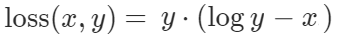
x represents the true label’s probability and y represents the predicted label’s probability.
When could it be used?
- Approximating complex functions
- Multi-class classification tasks
- If you want to make sure that the distribution of predictions is similar to that of training data
Example
import torch
import torch.nn as nn

input = torch.randn(2, 3, requires_grad=True)
target = torch.randn(2, 3)

kl_loss = nn.KLDivLoss(reduction = 'batchmean')
output = kl_loss(input, target)
output.backward()

print('input: ', input)
print('target: ', target)
print('output: ', output)
###################### OUTPUT ######################
input: tensor([[ 1.4676, -1.5014, -1.5201],
[ 1.8420, -0.8228, -0.3931]], requires_grad=True)
target: tensor([[ 0.0300, -1.7714, 0.8712],
[-1.7118, 0.9312, -1.9843]])
output: tensor(0.8774, grad_fn=<DivBackward0>)How to create a custom loss function in PyTorch?
PyTorch lets you create your own custom loss functions to implement in your projects.
Here’s how you can create your own simple Cross-Entropy Loss function.
Creating custom loss function as a python function
def myCustomLoss(my_outputs, my_labels):
    #specifying the batch size
    my_batch_size = my_outputs.size()[0]
    #calculating the log of softmax values
    my_outputs = F.log_softmax(my_outputs, dim=1)
    #selecting the values that correspond to labels
    my_outputs = my_outputs[range(my_batch_size), my_labels]
    #returning the results
    return -torch.sum(my_outputs)/number_examples
You can also create other advanced PyTorch custom loss functions.
Creating custom loss function with a class definition
Let’s modify the Dice coefficient, which computes the similarity between two samples, to act as a loss function for binary classification problems:
class DiceLoss(nn.Module):
    def __init__(self, weight=None, size_average=True):
        super(DiceLoss, self).__init__()

    def forward(self, inputs, targets, smooth=1):

        inputs = F.sigmoid(inputs)

        inputs = inputs.view(-1)
        targets = targets.view(-1)

        intersection = (inputs * targets).sum()
        dice = (2.*intersection + smooth)/(inputs.sum() + targets.sum() + smooth)

        return 1 - dice
How to monitor PyTorch loss functions?
It is quite obvious that while training a model, one needs to keep an eye on the loss function values to track the model’s performance. As the loss value keeps decreasing, the model keeps getting better. There are a number of ways that we can do this. Let’s take a look at them.
For this, we will be training a simple Neural Network created in PyTorch which will perform classification on the famous Iris dataset.
Making the required imports for getting the dataset.
from sklearn.datasets import load_iris
from sklearn.model_selection import train_test_split
from sklearn.preprocessing import StandardScaler
Loading the dataset.
iris = load_iris()
X = iris['data']
y = iris['target']
names = iris['target_names']
feature_names = iris['feature_names']
Scaling the dataset to have mean=0 and variance=1, gives quick model convergence.
scaler = StandardScaler()
X_scaled = scaler.fit_transform(X)
Splitting the dataset into train and test in an 80-20 ratio.
X_train, X_test, y_train, y_test = train_test_split(X_scaled, y, test_size=0.2, random_state=2)
Making the necessary imports for our Neural Network and its training.
import torch
import torch.nn.functional as F
import torch.nn as nn
import matplotlib.pyplot as plt
import numpy as np
plt.style.use('ggplot')
Defining our network.
class PyTorch_NN(nn.Module):
    def __init__(self, input_dim, output_dim):
        super(PyTorch_NN, self).__init__()
        self.input_layer = nn.Linear(input_dim, 128)
        self.hidden_layer = nn.Linear(128, 64)
        self.output_layer = nn.Linear(64, output_dim)

    def forward(self, x):
        x = F.relu(self.input_layer(x))
        x = F.relu(self.hidden_layer(x))
        x = F.softmax(self.output_layer(x), dim=1)
        return x
Defining functions for getting accuracy and training the network.
def get_accuracy(pred_arr,original_arr):
    pred_arr = pred_arr.detach().numpy()
    original_arr = original_arr.numpy()
    final_pred= []

    for i in range(len(pred_arr)):
        final_pred.append(np.argmax(pred_arr[i]))
    final_pred = np.array(final_pred)
    count = 0

    for i in range(len(original_arr)):
        if final_pred[i] == original_arr[i]:
            count+=1
    return count/len(final_pred)*100

def train_network(model, optimizer, criterion, X_train, y_train, X_test, y_test, num_epochs):
    train_loss=[]
    train_accuracy=[]
    test_accuracy=[]

    for epoch in range(num_epochs):

        #forward feed
        output_train = model(X_train)

        train_accuracy.append(get_accuracy(output_train, y_train))

        #calculate the loss
        loss = criterion(output_train, y_train)
        train_loss.append(loss.item())

        #clear out the gradients from the last step loss.backward()
        optimizer.zero_grad()

        #backward propagation: calculate gradients
        loss.backward()

        #update the weights
        optimizer.step()

        with torch.no_grad():
            output_test = model(X_test)
            test_accuracy.append(get_accuracy(output_test, y_test))

        if (epoch + 1) % 5 == 0:
            print(f"Epoch {epoch+1}/{num_epochs}, Train Loss: {loss.item():.4f}, Train Accuracy: {sum(train_accuracy)/len(train_accuracy):.2f}, Test Accuracy: {sum(test_accuracy)/len(test_accuracy):.2f}")

    return train_loss, train_accuracy, test_accuracy
Creating model, optimizer, and loss function object.
input_dim  = 4
output_dim = 3
learning_rate = 0.01

model = PyTorch_NN(input_dim, output_dim)
criterion = nn.CrossEntropyLoss()
optimizer = torch.optim.Adam(model.parameters(), lr=learning_rate)
1. Monitoring PyTorch loss in the notebook
Now you must have noticed the print statements in the train_network function to monitor the loss as well as accuracy. This is one way to do it.
X_train = torch.FloatTensor(X_train)
X_test = torch.FloatTensor(X_test)
y_train = torch.LongTensor(y_train)
y_test = torch.LongTensor(y_test)

train_loss, train_accuracy, test_accuracy = train_network(model=model, optimizer=optimizer, criterion=criterion, X_train=X_train, y_train=y_train, X_test=X_test, y_test=y_test, num_epochs=100)
We get an output like this.

If we want we can also plot these values using Matplotlib.
fig, (ax1, ax2, ax3) = plt.subplots(3, figsize=(12, 6), sharex=<strong>True</strong>)

ax1.plot(train_accuracy)
ax1.set_ylabel("training accuracy")

ax2.plot(train_loss)
ax2.set_ylabel("training loss")

ax3.plot(test_accuracy)
ax3.set_ylabel("test accuracy")

ax3.set_xlabel("epochs")
We would see a graph like this indicating the correlation between loss and accuracy.

This method is not bad and does the job. But we must remember that the more complex our problem statement and model get, the more sophisticated monitoring technique it would require.
2. Monitoring PyTorch loss with neptune.ai
A simpler way to monitor your metrics would be to log them in a service like Neptune, and focus on more important tasks, such as building and training the model.
To do this, we just need to follow a couple of small steps.
Note: For the most up-to-date code examples, please refer to the Neptune-PyTorch integration docs.
First, let’s install the required stuff.
pip install neptune-clientNow let’s initialize a Neptune run.
import neptune.new as neptune

run = neptune.init_run()
We can also assign config variables such as:
run["config/model"] = type(model).__name__
run["config/criterion"] = type(criterion).__name__
run["config/optimizer"] = type(optimizer).__name__
Here’s how it looks in the UI.

Finally, we can log our loss by adding just a couple of lines to our train_network function. Notice the ‘run’ associated lines.
def train_network(model, optimizer, criterion, X_train, y_train, X_test, y_test, num_epochs):
    train_loss=[]
    train_accuracy=[]
    test_accuracy=[]

    for epoch in range(num_epochs):

        #forward feed
        output_train = model(X_train)

        acc = get_accuracy(output_train, y_train)
        train_accuracy.append(acc)
        run["training/epoch/accuracy"].log(acc)

        #calculate the loss
        loss = criterion(output_train, y_train)
        run["training/epoch/loss"].log(loss)

        train_loss.append(loss.item())

        #clear out the gradients from the last step loss.backward()
        optimizer.zero_grad()

        #backward propagation: calculate gradients
        loss.backward()

        #update the weights
        optimizer.step()

        with torch.no_grad():
            output_test = model(X_test)
            test_acc = get_accuracy(output_test, y_test)
            test_accuracy.append(test_acc)

            run["test/epoch/accuracy"].log(test_acc)

        if (epoch + 1) % 5 == 0:
            print(f"Epoch {epoch+1}/{num_epochs}, Train Loss: {loss.item():.4f}, Train Accuracy: {sum(train_accuracy)/len(train_accuracy):.2f}, Test Accuracy: {sum(test_accuracy)/len(test_accuracy):.2f}")

    return train_loss, train_accuracy, test_accuracy
Here’s what we get in the dashboard. Absolutely seamless.

You can view this run here in the Neptune app. Needless to say, you can do this with any loss function.
Note: For the most up-to-date code examples, please refer to the Neptune-PyTorch integration docs.
Final thoughts
We went through the most common loss functions in PyTorch. You can choose any function that will fit your project, or create your own custom function.
Hopefully, this article will serve as your quick start guide to using PyTorch loss functions in your machine learning tasks.
If you want to immerse yourself more deeply into the subject or learn about other loss functions, you can visit the PyTorch official documentation.
打赏作者